An Introduction to R for
Watershed Ecology

R is a free programming language built for working with data. In watershed ecology, it can be used for almost everything: analyzing stream chemistry, estimating discharge, modeling nutrient loads, examining macroinvertebrate community composition, and producing publication-quality figures from monitoring data. By the end of this guide, you'll be able to do real watershed data analysis in R.

You don't need any programming experience. We'll go step by step, and there are exercises throughout to help you practice. Each exercise is followed by a worked solution so you can check your answer and understand the reasoning.

Two ways to use R

You have two options for working with R. Both run the same R language; the difference is where the code lives.

Right here in your browser. Every gray code cell on this page is a tiny live R session. Click Run and the code executes immediately, with output shown below the cell. You don't have to install anything. This is great for learning the language and working through this guide.

On your own computer with R and RStudio. For real work — projects, assignments, research — you'll want R installed locally so you can save your work, manage data files, and use the full suite of R packages. The rest of this chapter walks you through installing both pieces and explains how the desktop environment compares to the in-browser cells you'll use here.

Installing R and RStudio

You need two separate downloads. R is the language itself. RStudio is the editor you use to write and run R code. Install R first, then RStudio.

Step 1 — Install R

Go to cran.r-project.org (the Comprehensive R Archive Network). Pick the link that matches your operating system:

• Windows: Click "Download R for Windows" → "base" → "Download R-X.X.X for Windows". Run the installer with default settings.
• macOS: Click "Download R for macOS" and download the .pkg file matching your processor. Apple Silicon Macs (M1/M2/M3/M4) use the "arm64" build; older Intel Macs use the "x86_64" build. If you're not sure, click the Apple menu → About This Mac to check.
• Linux: Click "Download R for Linux" and follow the instructions for your distribution. On Ubuntu/Debian, the simplest command is sudo apt install r-base; on Fedora, sudo dnf install R. CRAN also has more recent builds maintained directly by the R project — check the page for your distribution.

Step 2 — Install RStudio

Go to posit.co/download/rstudio-desktop. (RStudio is now made by a company called Posit, but the software is still called RStudio.) The page should auto-detect your OS and show the right download. Run the installer.

Once both are installed, you only ever open RStudio — it finds and uses the R installation behind the scenes. You generally don't open R directly.

What RStudio looks like

When you open RStudio for the first time, you'll see a window divided into four panes. The screenshot below shows the typical layout:

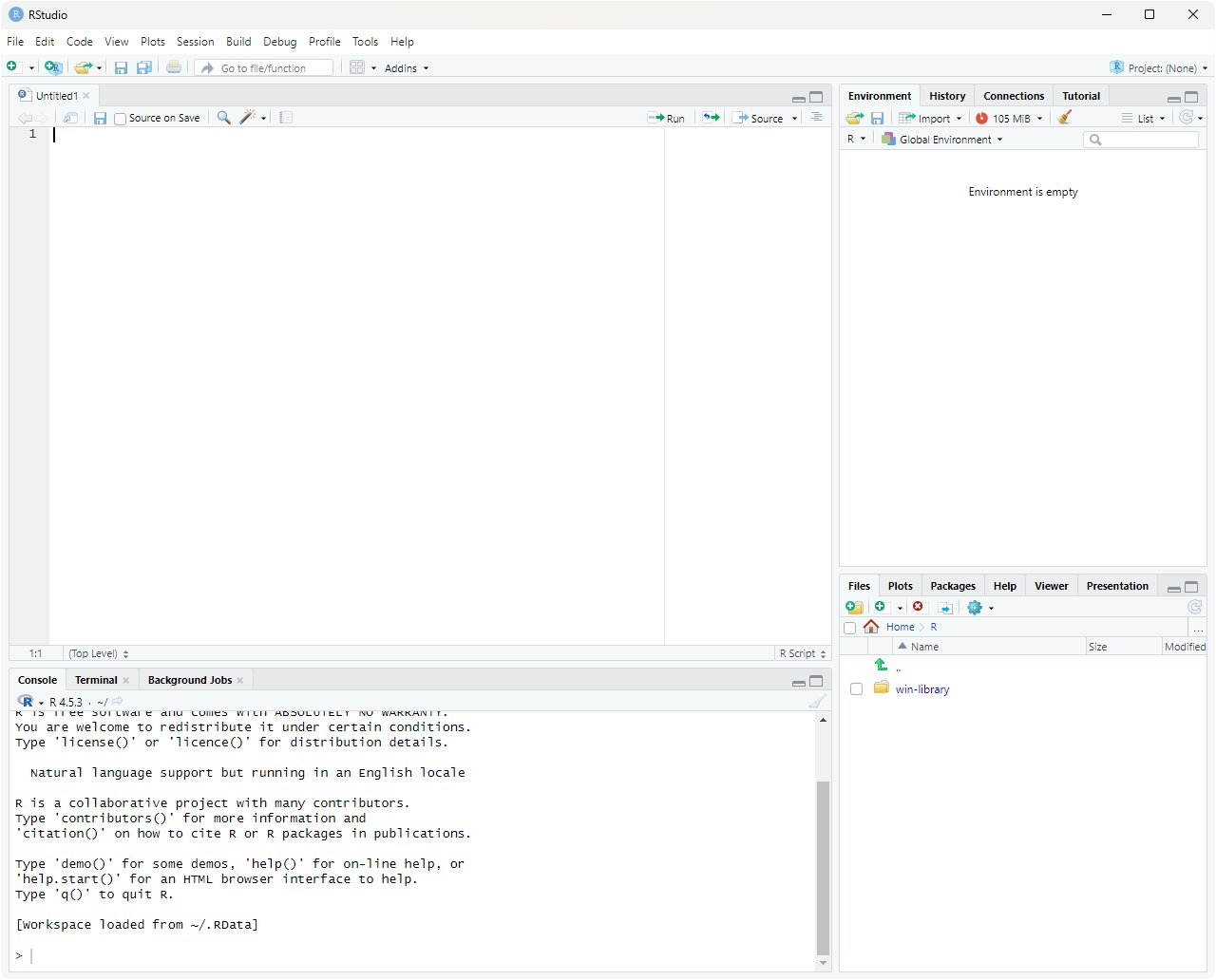
Each pane has a distinct job. Here's what they do:

1. Source editor (top-left) — where you write and save R scripts. A script is just a text file ending in .R that contains R code. You type code here and run it line-by-line (with Ctrl+Enter on Windows/Linux, Cmd+Return on Mac), or run the whole script at once.
2. Environment / History (top-right) — shows everything currently in memory. Variables, vectors, data frames you've created — all listed here with their values or dimensions. Think of it as a live inventory of your R session. Clicking a data frame opens it in a spreadsheet-style viewer, which is really helpful for inspecting datasets. The History tab shows every command you've ever typed in the current session.
3. Console (bottom-left) — the live R prompt. Anything you type here is executed immediately and the result appears right below. The console is what's actually running your R commands; the Source editor pane is just a place to write code that you then send to the console. When you click "Run" on a code cell on this webpage, you can think of it as sending that cell's contents to a hidden console.
4. Files / Plots / Help / Packages / Viewer (bottom-right) — a multi-purpose pane.
   • Files browses your project folder.
   • Plots displays figures you create with plot(), ggplot(), etc. — you can flip back through every plot you've made.
   • Help shows R's built-in documentation. Type ?mean in the console and the help page for mean() appears here.
   • Packages lists installed packages and lets you install new ones.
   • Viewer shows HTML output (knit reports, interactive widgets).

Projects and working directories

Once you start doing real analyses you'll have a folder full of related files: your R scripts, raw data, figures, and notes. Two RStudio concepts help you keep them organized.

The working directory. R has a notion of a "current folder" — the place it looks for files when you say things like read.csv("nitrate.csv"). That folder is called the working directory. You can ask R where it currently is with getwd(), and you can change it with setwd("/path/to/folder"). If R can't find a file you're trying to read, the most common reason is that your working directory is somewhere else and R is looking in the wrong place.

RStudio Projects. An RStudio Project is just a folder with a small .Rproj file inside it. When you open a project (File → Open Project, or by double-clicking the .Rproj file), three useful things happen:

• Your working directory is automatically set to the project folder. No more setwd() with hardcoded paths.
• RStudio remembers which scripts you had open last time, so you pick up where you left off.
• Variables you defined in your last session can optionally be restored.

The recommended workflow is: one project per analysis. For a class assignment, make a folder called something like watershed-assessment, create a new RStudio Project in it (File → New Project → New Directory), and put all your scripts and data inside. When you reopen the project a week later, you won't have to remember anything about where files live — R already knows.

A typical project folder might look like this:

• watershed-assessment/ — the project root
  • watershed-assessment.Rproj — the project file
  • data/ — raw data files (CSVs, shapefiles)
  • scripts/ — your .R analysis scripts
  • figures/ — plots you generate
  • README.md — a brief note describing the project

With this structure and a project file, references like read.csv("data/nitrate.csv") work the same on your laptop, your collaborator's laptop, and the lab computer. No absolute paths needed.

The R authoring environment

So far we've talked about R (the language) and RStudio (the editor). But when you start writing real analyses, you'll encounter a few more terms: IDE, R scripts, and R Markdown / Quarto documents. These are the three things that make up your day-to-day R workflow, and it's worth a quick tour before we head into the actual coding chapters.

RStudio is an IDE

RStudio is what's called an integrated development environment, or IDE for short. The name is more intimidating than the idea: an IDE is just a single application that bundles together the tools you need to write code. You've already seen the four panes — the source editor, the console, the environment viewer, and the files/plots/help pane. Each of those is a separate tool, but RStudio integrates them into one window so you don't have to juggle multiple programs.

Other languages have their own IDEs (VS Code, PyCharm, Eclipse, Xcode). For R, the dominant choice is RStudio. You could write R code in any plain text editor and run it from a terminal, but RStudio's tight integration of the console, plots, and help pages makes it dramatically more pleasant.

R scripts: the standard file format

An R script is a plain text file with the extension .R. It contains nothing but R code (and comments). When you run a script, R executes the lines from top to bottom as if you'd typed them into the console one at a time. Here's what a small script might look like:

Scripts are the right tool when your output is the analysis itself — a script that loads data, fits a model, and saves a figure to disk. They're the workhorses of reproducible research: anyone with the same data can run your .R file and get the same results. Most published analysis pipelines are built from one or more R scripts.

R Markdown and Quarto: writing with code

Sometimes the deliverable isn't just the analysis but a document — a lab report, a methods write-up, a thesis chapter. For these, plain R scripts aren't quite right because you also want explanations, headings, equations, figures, and tables, all woven together with the code that produced them.

That's what R Markdown (.Rmd files) and Quarto (.qmd files) are for. They're two closely-related formats — Quarto is Posit's newer, more flexible successor to R Markdown — that let you mix writing and code in one file. Quarto is increasingly the modern default, but the two work so similarly that you can treat them as one topic for now. We'll just call them "Rmd/Quarto" here.

Inside one of these files, prose is written as ordinary text (with markdown formatting for things like bold and headings), and R code lives in code chunks: small blocks fenced off by triple-backticks with {r} at the top. When you press Knit (for Rmd) or Render (for Quarto) in RStudio, the file is processed end-to-end: each code chunk runs, its output is captured (numbers, tables, figures), and everything is woven into a polished output document — usually HTML, PDF, or Word.

A typical chunk inside an Rmd/Quarto file looks like this:

For example: a watershed assessment lab report might have an introduction paragraph, a code chunk that loads the field data, another paragraph describing the analysis, a chunk that fits a linear model and prints the summary, then a chunk that produces a final figure — all in one .Rmd or .qmd file. When you knit it, the result is a single PDF or HTML document with the prose flowing naturally around the figures and tables generated by your code. No copy-pasting between R and Word. If the data updates, you just re-knit and everything regenerates.

How this webpage compares to all of the above

The code cells you'll use throughout this guide sit in an interesting middle ground. Conceptually, they're closest to Rmd/Quarto chunks — prose and runnable R code interleaved on a page — except that this page is fixed and you don't render anything. Compared to working in RStudio with real .R or .qmd files, the code cells here are intentionally simpler:

• Persistence between cells. Each cell on this webpage runs in a fresh R environment, so variables you create in one cell are not automatically available in the next — that's why some exercises ask you to recreate a data frame at the top of your answer. In RStudio (script or notebook), your variables persist for the entire session.
• Saving your work. Code typed into a cell here lives only as long as the browser tab is open. .R, .Rmd, and .qmd files all save to your computer where you can edit, version-control with git, and share them.
• Packages. Only a handful of R packages are pre-loaded in your browser (we have ggplot2, but not the full tidyverse). In RStudio you can install any of the ~20,000 packages on CRAN with a single command.
• Data files. The cells here can't read CSVs or other files from your hard drive. In RStudio you'll routinely use read.csv(), read_csv(), or specialized functions like dataRetrieval::readNWISdv() to pull discharge records straight from the USGS.
• Knitting / rendering. This page is hand-written HTML; nothing gets rendered from a source document. With Rmd/Quarto, the file you write is the source — you knit it whenever you want to produce the final output.
• Speed. The browser version downloads R-compiled-to-WebAssembly the first time you visit, which takes ~30 seconds. R running locally through RStudio is at native speed once installed.

The code cells here are good enough to work through this guide — you can focus on learning R without worrying about installation, file paths, or knitting. Once you're ready to do your own analyses, you'll likely use R scripts for the analysis itself and .Rmd/.qmd documents to write up the results. The beauty is that the R syntax you learn here works identically in all three.

Before you write your first line of R, a few vocabulary words will save you a lot of confusion. This short chapter introduces four terms — code, comments, functions, and operators — that show up on every page of this guide.

Code and Comments

Code is just text — instructions written for the computer to follow. Each line tells R to do something specific. R reads your code top to bottom, one line at a time, and does exactly what you say. If R does something unexpected, it's because the code told it to. Reading the line carefully is almost always the first step in fixing a bug (or, problem in the code).

Lines that start with # are comments — notes for humans that R ignores completely. Comments are how you explain to your future self (or classmate/professor/colleague) what your code is doing:

Functions

A function is a named procedure that takes one or more inputs and gives back a result. You can think of a function like a labeled machine: you put something in, the machine does its job, and something comes out. R comes with thousands of functions built in, and you'll learn many of them throughout this guide.

You "call" (run) a function by writing its name followed by parentheses. Whatever you put inside the parentheses is the input (sometimes called an argument). For example, sqrt() is the square-root function:

The parentheses are essential. sqrt(16) calls the function on 16, but sqrt by itself just refers to the function as an object — like saying the word "calculator" instead of actually using one. Forgetting parentheses, or having them in the wrong place, is a common source of error for beginners.

You'll see this same pattern everywhere in R. mean(x) takes a vector x and gives back its average. length(x) gives you how many items are in x. read.csv("nitrate.csv") reads a CSV file. The pattern is always function-name followed by parentheses around the input.

Arguments aren't always required for a function (e.g., getwd() is a function that returns your current working directory). Sometimes arguments have default values, so you don't have to specify them each time. If you're curious about the arguments a function accepts, you can use the help function ?function_name to view its documentation.

Operators

An operator is a special shortcut symbol that acts like a tiny function. You've used them in math your whole life: +, -, *, /. R has the same arithmetic operators, plus a few R-specific ones like <- (used to store values in variables, which we'll see in the next chapter) and == (which checks whether two things are equal).

Operators don't use parentheses around their inputs — they sit between them. So 2 + 3 is an operator (+) acting on two numbers, while sum(2, 3) is a function (sum) acting on two numbers. Both give 5; the syntax is just different.

That's the whole vocabulary you need to start reading R code: code is what you type, comments are notes for humans, functions are named procedures called with parentheses, and operators are shortcut symbols.

A variable is a named container that holds a value. Once you store something in a variable, you can refer to it by name in later calculations. This saves typing and makes your code easier to read.

In R, we assign values using the arrow operator <- or the equals sign =. Read it as "gets":

You can use variables in calculations:

Naming rules

Variable names should be descriptive. nitrate_mg_per_L is far better than x because anyone reading your code (including future-you) will know what it means. A few rules:

• Names can contain letters, numbers, dots, and underscores
• Names must start with a letter
• R is case-sensitive: Discharge and discharge are different variables
• Avoid using names of built-in functions like mean, sum, or c

In watershed ecology, you almost never make just one measurement — you sample across sites, dates, or depths. A vector is an ordered list of values of the same type (all numbers, or all text). You build vectors with the c() function, which stands for "combine."

Math on vectors

R applies math operations to every element of a vector at once. This is called vectorization, and it's one of the most powerful features of R:

Pulling out specific values

Use square brackets [ ] to access individual elements. R indexes from 1 (not 0):

You can also pull out values that meet a condition. This is called logical subsetting:

A data frame is R's version of a spreadsheet. It has rows (typically one per sample, site, or sampling date) and columns (one per measurement or variable). Data frames are the workhorse of data analysis.

Let's build a small data frame from a hypothetical synoptic stream survey:

The ept_taxa column counts the number of Ephemeroptera, Plecoptera, and Trichoptera (mayfly, stonefly, and caddisfly) taxa — a common bioindicator where higher numbers generally suggest better water quality.

Inspecting a data frame

Real datasets often have hundreds or thousands of rows, so you usually want a quick look rather than the whole thing:

Accessing columns and filtering rows

Use the dollar sign $ to grab a single column:

The & symbol means "AND" (both conditions must be true). The | symbol means "OR" (either can be true).

Arithmetic operators

Comparison operators

These return TRUE or FALSE:

Logical operators

Watershed ecology is full of equations — runoff models, nutrient load calculations, dilution equations, hydraulic geometry relationships. A core R skill is taking an equation off a textbook page and turning it into working code.

Manning's equation for open-channel flow

v = (1/n) · R^2/3 · S^1/2

where v is mean velocity (m/s), n is Manning's roughness coefficient, R is hydraulic radius (m), and S is the channel slope (m/m).

Pollutant load calculation

L = C × Q × k

where L is load (kg/day), C is concentration (mg/L), Q is discharge (m³/s), and k is the unit conversion factor 86.4.

Because columns are vectors, you can do math across an entire column in one line — no loops needed. R automatically applies the operation row by row.

In four lines of code, we computed four new variables for all ten sites at once. If the dataset had 10,000 sites, the code would be exactly the same.

A for loop runs a block of code once for each item in a sequence. Use it when you know in advance what set of values you want to iterate over — a list of sites, a series of years, a vector of measurements. (Use a while loop, which we'll see in the next chapter, when you don't know how many iterations you'll need.)

The syntax reads almost like English: for (each item in my_list) do something with item:

Inside the parentheses, i is a variable name we chose — it takes on each value of the sequence 1:5 in turn. You can name the loop variable anything you like (often i or j for indices, or something descriptive like site or year).

A watershed example: looping over sites

Suppose you have a vector of stream site names and you want to print a quick status report for each one:

The loop variable site takes on each character string in turn. The paste() function glues strings together with a space between them.

Building up a result inside a loop

A common pattern is to start with an empty container, then accumulate values as the loop runs. Here we compute a running total of monthly precipitation, recording the cumulative total after each month:

Notice the pattern: we initialized running_total as an empty numeric vector with the right length, set the first element by hand, then used the loop to fill in each subsequent element by adding the next month's precipitation to the previous total. This kind of iterative accumulation is the bread and butter of for loops.

A while loop runs a block of code repeatedly as long as a condition stays true. It's the right tool when you don't know in advance how many iterations you'll need — you just know when to stop.

A watershed example: simulating a reservoir filling

A small reservoir starts at 40% capacity. Inflows raise its level by 4 percentage points per day during a wet period. How many days until it reaches at least 95%?

A linear model describes the relationship between a response variable and one or more predictor variables. R fits linear models with the lm() function. The syntax y ~ x reads as "y is modeled as a function of x."

Stage-discharge rating curve

The relationship between stream stage and discharge typically follows a power law Q = a · h^b, which becomes linear after taking logs of both sides:

log(Q) = log(a) + b · log(h)

R has plotting tools built right into the language. Plots produced in code cells appear below the cell as images.

Boxplots compare distributions across groups

ggplot2 uses a layered approach — you start with a blank canvas, map data to visual elements, then add geoms (points, lines, bars), labels, and themes with the + operator.

Let's combine everything you've learned into a mini analysis. We'll simulate a synoptic stream survey, compute derived metrics, fit a stressor-response model, and visualize the results.

This 30-line analysis touches every concept from the guide: variables, vectors, data frames, operators, equations, column-wise math, while loops, linear models, and plotting. Real watershed analyses are just longer versions of this same pattern — and the stressor-response framework you see here is essentially the foundation of state and federal assessment programs.